The memory wall: compute outpaces off-chip memory bandwidth.
The memory wall problem
- Processor compute capability grows ~50% per year; DRAM bandwidth grows ~7-10% per year.
- Modern GPUs/accelerators demand >1 TB/s of memory bandwidth for AI/ML workloads.
- HBM (High Bandwidth Memory) addresses this through 3D-stacked DRAM + wide I/O interfaces.
- 2.5D integration uses a silicon interposer to place HBM and processor side-by-side.
Our approach
We use DRAMsim3 to systematically compare architectures and understand which parameters truly matter — not just peak bandwidth, but achieved bandwidth, latency, utilization, and energy.
A unified DRAMsim3 workflow connects architectures, workloads, and metrics.
Experimental setup
- Simulator: DRAMsim3 (cycle-accurate, open source).
- Architectures: DDR4 baseline, HBM baseline, HMC/2.5D proxy.
- HBM sensitivity: channels (1/2/4/8), frequency (800/1000/1250/2000 MHz), queue size (16/32/64).
- Workloads: built-in stream (high locality) & random (low locality); timed synthetic traces (light/mixed/heavy) for DVFS.
Metrics
- Achieved bandwidth (GB/s)
- Average read latency (ns)
- Bandwidth utilization = achieved / peak
- Energy per completed request (pJ/req)
- DVFS: energy saving %, EDP improvement %, bandwidth/latency change %
Three architectures compared under controlled workloads.
| Architecture | Config source | Key characteristics | Role |
|---|---|---|---|
| DDR4 | DDR4_Baseline.ini |
1 channel, 64-bit bus, ~101.6 GB/s peak | Conventional memory baseline |
| HBM | HBM_Baseline.ini |
8 channels, 128-bit per channel, 4 dies, ~512 GB/s peak | Main target: stacked wide-I/O memory |
| HMC/2.5D proxy | HMC_4GB_4Lx16.ini |
16 channels (4 links × 16 lanes), ~120 GB/s peak | Proxy for 2.5D stacked/interposer memory |
Workloads
Stream: sequential, row-buffer-friendly → tests peak bandwidth capability.
Random: uniform random, low locality → tests latency and queue behavior.
Experiment design principle
Each architecture runs both workloads for 200,000 cycles. We record achieved BW, average read latency, bandwidth utilization, and energy per request — all from the same DRAMsim3 output parser.
HBM delivers 10.43x stream and 3.27x random bandwidth over DDR4.
| Metric | Workload | DDR4 | HBM | HMC/2.5D | HBM/DDR4 | HMC/HBM |
|---|---|---|---|---|---|---|
| Achieved BW (GB/s) | Stream | 16.9 | 176.4 | 110.6 | 10.43x | 0.63x |
| Random | 18.5 | 60.6 | 79.9 | 3.27x | 1.32x | |
| Avg Read Latency (ns) | Stream | 248.6 | 75.0 | 229.0 | 0.30x | 3.05x |
| Random | 484.5 | 380.7 | 93.1 | 0.79x | 0.24x | |
| Energy/Request (pJ) | Stream | 11178 | 1152 | 1059 | 0.10x | 0.92x |
| Random | 17299 | 2400 | 1196 | 0.14x | 0.50x |
Key finding 1
HBM dominates stream workloads — 10.43x bandwidth, dramatically lower latency and energy. The wide channel interface and channel-level parallelism convert peak BW into achieved BW.
Key finding 2
HMC/2.5D proxy gives better random access performance than HBM (1.32x BW, 93ns vs 381ns latency). This suggests a different latency-bandwidth tradeoff in 2.5D-style architectures.
Three HBM parameters varied one at a time: channels, frequency, queue size.
| Parameter | Values tested | What it reveals | Significance |
|---|---|---|---|
| Channel count | 1, 2, 4, 8 | Channel-level parallelism; queue pressure distribution | Strongest result |
| Frequency (MHz) | 800, 1000, 1250, 2000 | Peak BW vs. achieved BW; diminishing returns; DRAM bottleneck hypothesis | Focus of this section |
| Transaction queue size | 16, 32, 64 | Memory-level parallelism exploitation | Workload-dependent |
Stream BW grows but saturates; random BW is nearly flat above 1000 MHz.
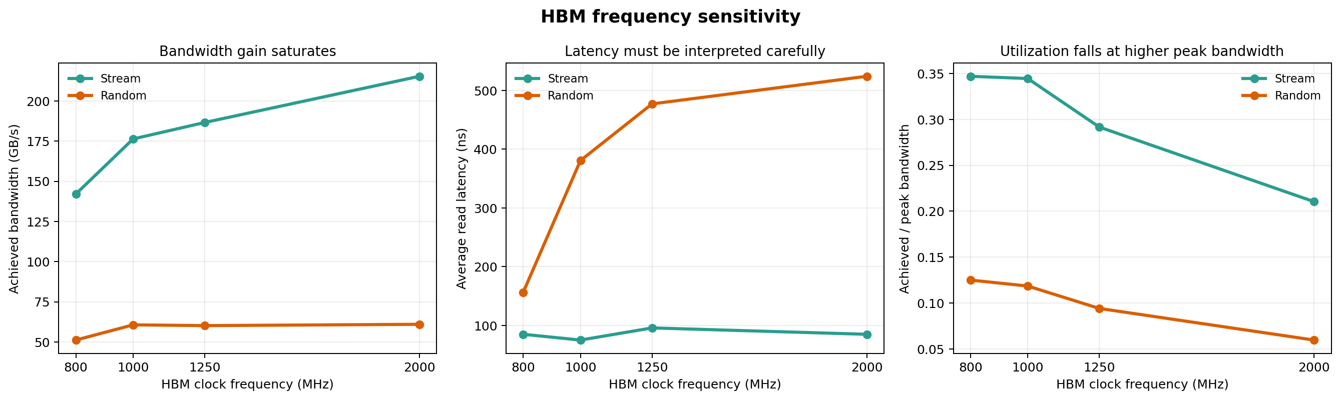
| Frequency (MHz) | Peak BW (GB/s) | Stream BW (GB/s) | Random BW (GB/s) | Stream Util. | Random Util. | Random Latency (ns) |
|---|---|---|---|---|---|---|
| 800 | 409.6 | 142.1 | 51.1 | 34.7% | 12.5% | 156.2 |
| 1000 | 512.0 | 176.4 | 60.6 | 34.4% | 11.8% | 380.7 |
| 1250 | 640.0 | 186.6 | 60.1 | 29.2% | 9.4% | 477.1 |
| 2000 | 1024.0 | 215.4 | 61.0 | 21.0% | 6.0% | 524.1 |
Why does random bandwidth saturate? The DRAM core timing is the bottleneck.
Stream workload: partial scaling
- BW grows from 142.1 → 215.4 GB/s (+51.6% across 800→2000 MHz).
- But utilization drops from 34.7% → 21.0%.
- Peak BW grows 2.5x (409.6→1024 GB/s), achieved BW grows only 1.5x.
- Diminishing returns: each frequency increment converts less into achieved BW.
- Energy/request grows from 917 → 2656 pJ (+190%) — significant energy cost.
Random workload: complete saturation
- BW is essentially flat: 51.1 → 61.0 GB/s at 800→2000 MHz (+19%).
- Above 1000 MHz: zero gain (60.6 → 60.1 → 61.0 GB/s).
- Utilization collapses: 12.5% → 6.0%.
- Latency increases from 156 → 524 ns (3.4x).
- Energy/request explodes from 1786 → 7784 pJ (+336%).
Key takeaways: frequency is not a free lunch.
3 conclusions from frequency sensitivity
- Stream benefits but with diminishing returns. Each extra MHz of peak BW converts less efficiently into achieved BW. The sweet spot appears around 1000 MHz (34.4% utilization, 176.4 GB/s).
- Random BW is DRAM-core-limited. Above 1000 MHz, the interface can deliver more, but the DRAM timing (tRCD + CL + tRP) cannot service random requests any faster. Adding more peak BW is wasted.
- Higher frequency costs energy proportionally more than it delivers bandwidth. For random: +150% peak BW (1000→2000) costs +63% energy per request with +0.6% bandwidth gain.
This directly motivates our new experiment
If DRAM core timing is the real bottleneck for random access, can we prove this by varying DRAM timing parameters (tRCD, tRP, tCL) directly? → See Part 3(c): DRAM as Bottleneck.
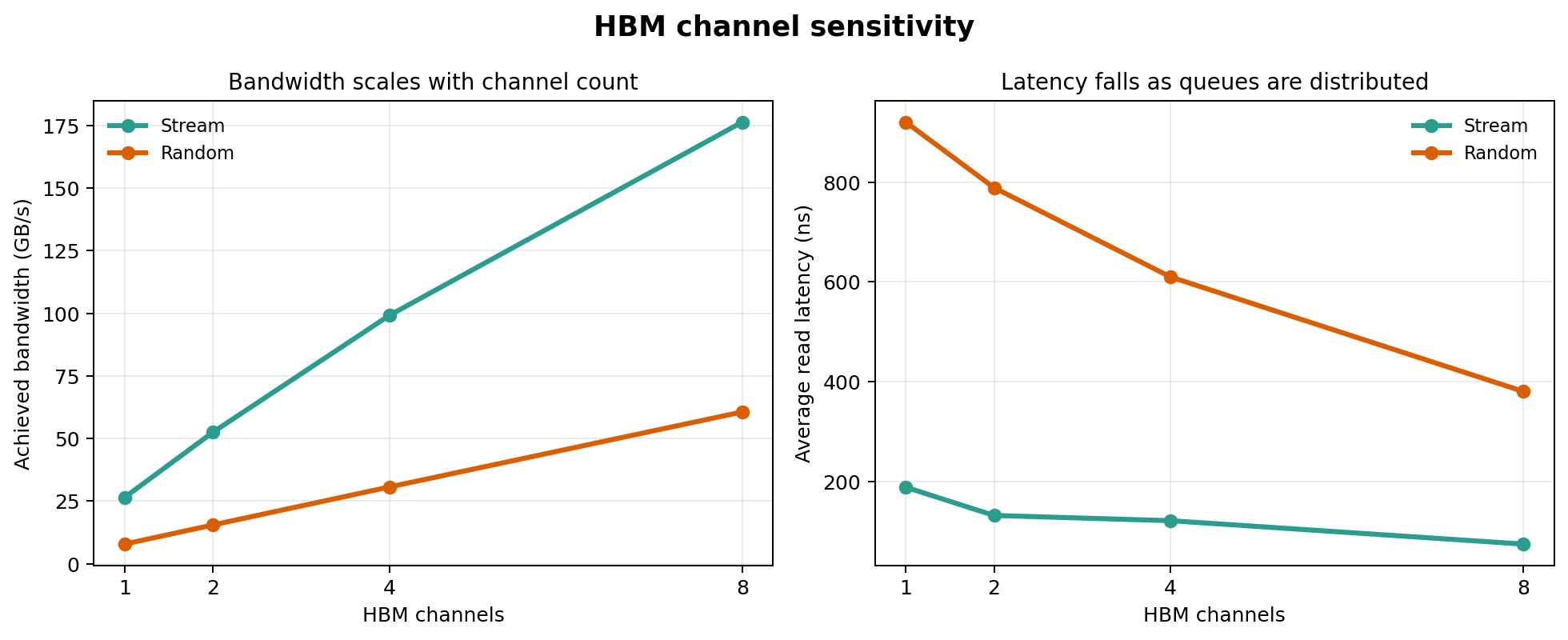
Channel count is the most reliable HBM tuning dimension.
Bandwidth scaling
- Stream: 26.5 → 176.4 GB/s = 6.66x from 1→8 channels
- Random: 7.8 → 60.6 GB/s = 7.73x from 1→8 channels
- Near-linear scaling: channels expose independent memory-level parallelism
Latency reduction
- Stream: 188.9 → 75.0 ns = 60% reduction
- Random: 920.3 → 380.7 ns = 59% reduction
- Queue pressure distributes across channels → lower per-channel contention
Larger queues help stream (1.62x) but not random (1.01x).
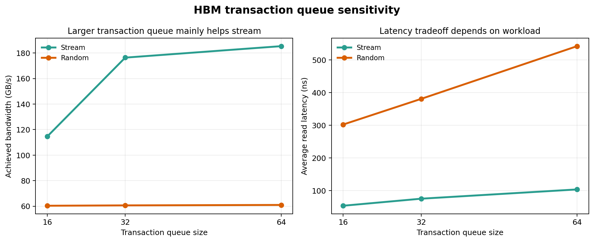
| Queue size | Stream BW (GB/s) | Random BW (GB/s) | Stream Latency (ns) | Random Latency (ns) |
|---|---|---|---|---|
| 16 | 114.6 | 60.3 | 53.4 | 302.1 |
| 32 | 176.4 | 60.6 | 75.0 | 380.7 |
| 64 | 185.4 | 61.0 | 103.3 | 542.1 |
Interpretation
Queue capacity exposes memory-level parallelism. Stream benefits because its sequential access pattern has exploitable parallelism — more outstanding requests can be pipelined across banks and channels. Random does not benefit because each request is structurally independent and the bottleneck is DRAM timing, not queue depth. Larger queues trade latency for throughput: at queue=64, stream latency rises +36% but BW gains only +5.1% over queue=32.
Load-aware frequency switching saves energy when the workload leaves slack.
Method
- Split timed traces into 100K-cycle windows
- Baseline probe: measure load index L ∈ [0,1] per window at 1250 MHz
- Decision: L < 0.4 → 800 MHz, L < 0.7 → 1000 MHz, else → 1250 MHz
- Simulate each window at selected frequency, aggregate results
4 workload scenarios
- Light: sparse random, gap 200-800 cycles, L~0.2
- Mixed: alternating dense/sparse phases, L∈[0.3,0.8]
- Heavy: dense random with 20% priority requests, L>0.7
- Baseline: dense random, no priority, L>0.7
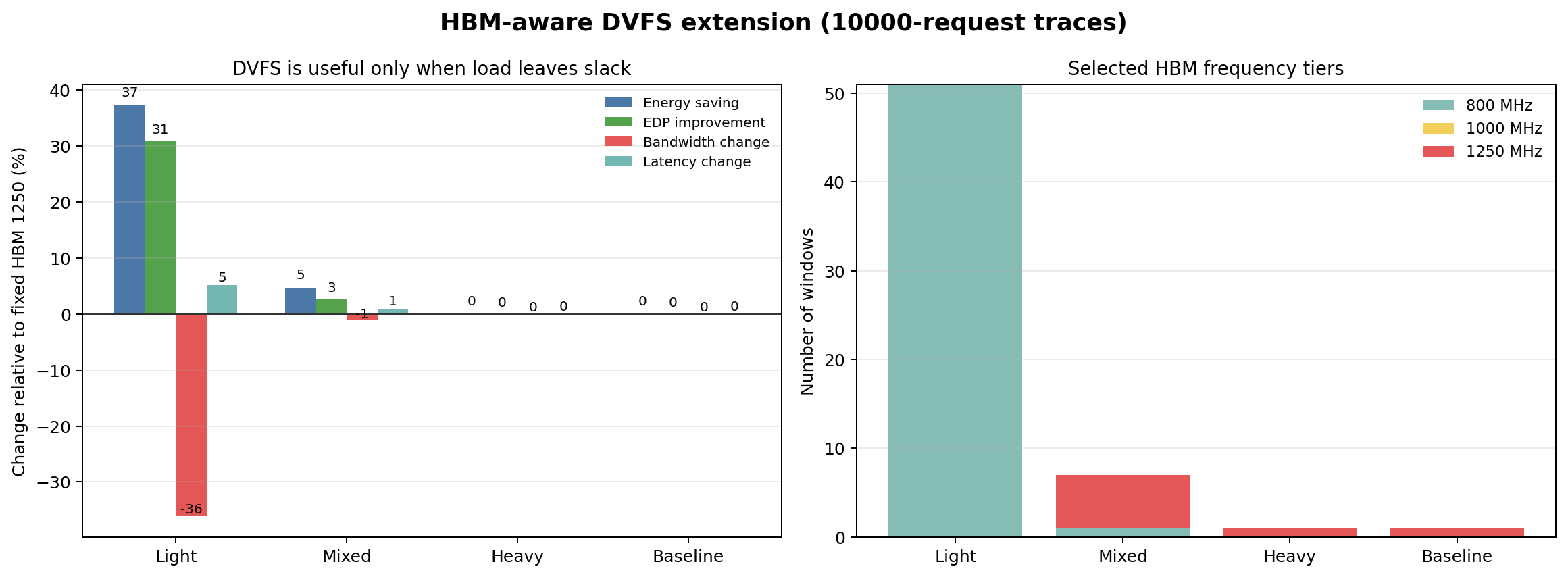
DVFS saves 37.3% energy at light load, with 30.8% EDP improvement.
| Scenario | Energy Saving | EDP Improvement | BW Change | Latency Change | 800 MHz wins | 1250 MHz wins | Verdict |
|---|---|---|---|---|---|---|---|
| Light | 37.3% | 30.8% | -36.1% | +5.2% | 51 | 0 | Ideal tradeoff |
| Mixed | 4.7% | 2.6% | -1.1% | +1.0% | 1 | 6 | Modest benefit |
| Heavy | 0% | 0% | 0% | 0% | 0 | 1 | Correctly stays high |
| Baseline | 0% | 0% | 0% | 0% | 0 | 1 | Correctly stays high |
When is the tradeoff ideal?
Light workloads (L < 0.4): 37.3% energy saving, 30.8% EDP improvement, only 5.2% latency increase. The 36.1% bandwidth loss is acceptable because the workload doesn't need it. All 51 windows run at 800 MHz — the policy correctly identifies sustained low load.
When is DVFS not useful?
Heavy/sustained workloads: the policy correctly holds at 1250 MHz, claiming no artificial savings. Mixed workloads: modest 4.7% energy saving — the sparse windows are too few to accumulate significant savings.
2.5D integration trades stream bandwidth for better random access latency.
What is 2.5D stacked HBM?
2.5D integration places HBM stacks and the processor die side-by-side on a silicon interposer. The interposer provides ultra-dense routing (~2μm pitch vs. ~100μm on PCB), enabling thousands of short, low-power connections between memory and processor.
- HBM dies are 3D-stacked with TSVs (through-silicon vias)
- The stack sits on a base logic die connected to the interposer
- Interposer routes signals from HBM to processor with minimal distance (~2-5mm)
- Key benefit: shorter physical path → lower latency, lower power per bit
Our proxy: HMC/2.5D in DRAMsim3
We use the HMC (Hybrid Memory Cube) configuration as a proxy for 2.5D-style stacked memory. HMC shares key characteristics: 3D-stacked DRAM, serialized links through a logic base, and proximity to the processor via interposer-style connection. Caveat: DRAMsim3 does not model physical interposer routing delay or thermal effects.
Why this tradeoff?
HMC uses 16 narrow serial links (4 links × 16 lanes) instead of HBM's 8 wide parallel channels. The serialized, packet-based protocol has lower per-access overhead for random requests, but lower peak streaming bandwidth. This creates an architecture-consistent tradeoff: 2.5D/HMC is better for latency-sensitive, irregular workloads; HBM is better for bandwidth-hungry, regular workloads.
Proving that DRAM timing — not interface bandwidth — limits random access.
Motivation from existing data
Our frequency sweep showed random BW saturating at ~61 GB/s regardless of interface frequency (1000→2000 MHz: zero gain). This strongly suggests the bottleneck is not the HBM interface but the DRAM core timing parameters. Every random access pays tRCD (row activation) + CL (column read) + tRP (precharge), which are fixed real-time costs independent of interface speed.
Hypothesis: In random-access workloads, DRAM row cycle time (tRC = tRAS + tRP) dominates overall latency, making interface bandwidth irrelevant beyond a threshold.
Experiment design space: 3 proposals
(Choose one or combine; suggested priority order shown)
Proposal 1 (Recommended): Systematically vary DRAM core timing parameters
Setup: Fix HBM at 1250 MHz (8 channels, queue=32). Create 5 configs where tRCD, tRP, tCL are scaled by 0.5x / 0.75x / 1.0x / 1.5x / 2.0x relative to baseline.
Metrics: Achieved random BW, random latency, utilization.
Prediction: If DRAM core is the bottleneck, slowing timing by 2x should approximately halve random BW, while speeding by 2x should nearly double it. If interface is the bottleneck, changes will have minimal effect.
HBM_1250_tRCD_0p5x.ini through HBM_1250_tRCD_2p0x.ini
Proposal 2: Row buffer locality sweep (tRC bottleneck proof)
Setup: Create 5 traces with controlled row buffer hit rates: 0%, 25%, 50%, 75%, 100%. Simulate at HBM 1250 MHz (8 channels).
Prediction: BW should scale linearly with row hit rate, because each miss costs the full tRC (row close + open). At 0% hit rate, even HBM's peak BW is irrelevant — the DRAM core tRC determines maximum throughput.
Key formula: Max random BW ≈ (bus width × channels) / tRC when row hit rate = 0.
Proposal 3: Bank count sensitivity (find bank-level parallelism limit)
Setup: Vary HBM bank groups (2/4/8) and banks per group (2/4/8) at fixed 1250 MHz. Total banks: 4, 8, 16, 32, 64.
Prediction: Random BW should saturate when #banks > #outstanding random requests that can be serviced in parallel. This identifies the bank-level parallelism ceiling.
Strongest conclusions come from being clear about what we do not claim.
What we do NOT claim
- The HMC/2.5D result is a proxy — it does not model physical interposer routing, thermal, or distance effects.
- Frequency sensitivity is affected by cycle-driven workload generation; do not generalize "higher frequency = slower random" as a universal law.
- DVFS does not support P99 latency, SLA violation rate, or tail-latency guarantees.
- Synthetic stream/random workloads show architectural sensitivity, not full application speedup.
- DRAM core bottleneck experiment (Part 3c) is proposed but not yet executed.
Future work directions
- Execute DRAM bottleneck experiment (Proposal 1: timing parameter sweep).
- Add per-request latency logging for P99/tail analysis in DVFS.
- Use application-derived memory traces (e.g., SPEC, ML benchmarks).
- Model interposer effects more explicitly or cross-validate with another simulator.
- Explore 3D-stacked HBM (HBM3/HBM3e) with more channels and higher frequencies.
HBM's value comes from converting architecture resources into achieved bandwidth — and knowing what limits that conversion.
Baseline
HBM strongly outperforms DDR4. The advantage is workload-dependent: 10.43x stream, 3.27x random.
Sensitivity
Channels are the most reliable tuning dimension. Frequency has diminishing returns; random BW hits a DRAM core ceiling.
Innovation
DVFS saves energy when load is low. 2.5D changes the latency/BW tradeoff. DRAM bottleneck experiment will quantify the core timing limit.